


Do you want to analyze data that resides in Google BigQuery as part of an R workflow? Thanks to the bigrquery R package, it’s a pretty seamless experience — once you know a couple of small tweaks needed to run dplyr functions on such data.
First, though, you’ll need a Google Cloud account. Note that you’ll need your own Google Cloud account even if the data is in someone else’s account and you don’t plan on storing your own data.
How to set up a Google Cloud account
Many people already have general Google accounts for use with services like Google Drive or Gmail. If you don’t have one yet, make sure to create one.
Then, head to the Google Cloud Console at https://console.cloud.google.com, log in with your Google account, and create a new cloud project. R veterans note: While projects are a good idea when working in RStudio, they’re mandatory in Google Cloud.
 Screenshot by Sharon Machlis, IDG
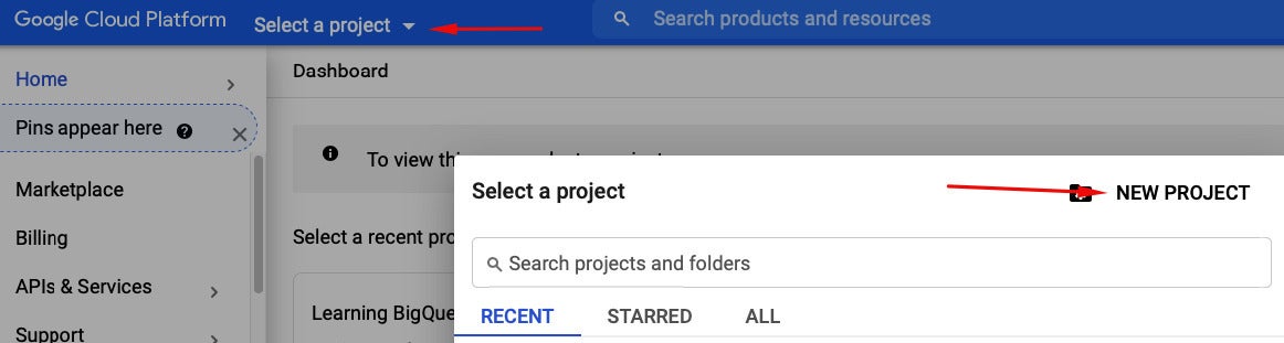
Click the New Project option in order to create a new project.
You should see the option to create a new project at the left side of Google Cloud’s top navigation bar. Click on the dropdown menu to the right of “Google Cloud Platform” (it might say “select project” if you don’t have any projects already). Give your project a name. If you have billing enabled already in your Google account you’ll be required to select a billing account; if you don’t, that probably won’t appear as an option. Then click ”Create.”
 Screenshot by Sharon Machlis, IDG
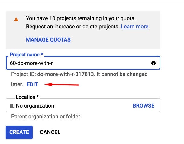
If you don’t like the default project ID assigned to your project, you can edit it before clicking the Create button.
If you don’t like the project ID that is automatically generated for your project, you can edit it, assuming you don’t pick something that is already taken.
Make BigQuery easier to find
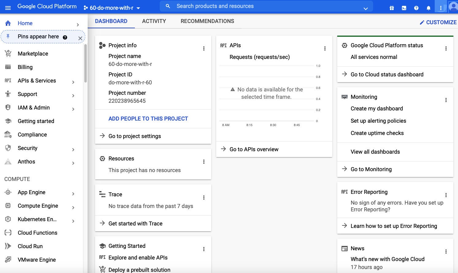
Once you finish your new project setup, you’ll see a general Google Cloud dashboard that may seem a bit overwhelming. What are all these things and where is BigQuery? You probably don’t need to worry about most of the other services, but you do want to be able to easily find BigQuery in the midst of them all.
 Screenshot by Sharon Machlis, IDG
The initial Google Cloud home screen can be a bit overwhelming if you are looking to use just one service. (I’ve since deleted this project.)
One way is to “pin” BigQuery to the top of your left navigation menu. (If you don’t see a left nav, click the three-line “hamburger” at the very top left to open it.) Scroll all of the way down, find BigQuery, hover your mouse over it until you see a pin icon, and click the pin.
 Screenshot by Sharon Machlis, IDG
Scroll down to the bottom of the left navigation in the main Google Cloud home screen to find the BigQuery service. You can “pin” it by mousing over until you see the pin icon and then clicking on it.
Now BigQuery will always show up at the top of your Google Cloud Console left navigation menu. Scroll back up and you’ll see BigQuery. Click on it, and you’ll get to the BigQuery console with the name of your project and no data inside.
If the Editor tab isn’t immediately visible, click on the “Compose New Query” button at the top right.
Start playing with public data
Now what? People often start learning BigQuery by playing with an available public data set. You can pin other users’ public data projects to your own project, including a suite of data sets collected by Google. If you go to this URL in the same BigQuery browser tab you’ve been working in, the Google public data project should automatically pin itself to your project.
Thanks to JohannesNE on GitHub for this tip: You can pin any data set you can access by using the URL structure shown below.
https://console.cloud.google.com/bigquery?p={project-id}&page=projectIf this doesn’t work, check to make sure you’re in the right Google account. If you’ve logged into more than one Google account in a browser, you may have been sent to a different account than you expected.
After pinning a project, click on the triangle to the left of the name of that pinned project (in this case bigquery-public-data) and you’ll see all data sets available in that project. A BigQuery data set is like a conventional database: It has one or more data tables. Click on the triangle next to a data set to see the tables it contains.
 Screenshot by Sharon Machlis, IDG
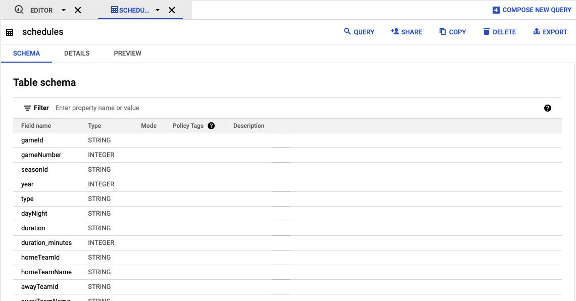
Clicking on a table in the BigQuery web interface lets you see its schema, along with a tab for previewing data.
Click on the table name to see its schema. There is also a “Preview” tab that lets you view some actual data.
There are other, less point-and-click ways to see your data structure. But first....
How BigQuery pricing works
BigQuery charges for both data storage and data queries. When using a data set created by someone else, they pay for the storage. If you create and store your own data in BigQuery, you pay — and the rate is the same whether you are the only one using it, you share it with a few other people, or you make it public. (You get 10 GB of free storage per month.)
Note that if you run analysis on someone else’s data and store the results in BigQuery, the new table becomes part of your storage allocation.
Watch your query costs!
The price of a query is based on how much data the query processes and not how much data is returned. This is important. If your query returns only the top 10 results after analyzing a 4 GB data set, the query will still use 4 GB of your data analysis quota, not simply the tiny amount related to your 10 rows of results.
You get 1 TB of data queries free each month; each additional TB of data processed for analysis costs $5.
If you’re running SQL queries directly on the data, Google advises never running a SELECT * command, which goes through all available columns. Instead, SELECT only the specific columns you need to cut down on the data that needs to be processed. This not only keeps your costs down; it also makes your queries run faster. I do the same with my R dplyr queries, and make sure to select only the columns I need.
If you’re wondering how you can possibly know how much data your query will use before it runs, there’s an easy answer. In the BigQuery cloud editor, you can type a query without running it and then see how much data it will process, as shown in the screenshot below.
 Screenshot by Sharon Machlis, IDG
Using the BigQuery SQL editor in the web interface, you can find your table under its data set and project. Typing in a query without running it shows how much data it will process. Remember to use `projectname.datasetname.tablename` in your query
Even if you don’t know SQL, you can do a simple SQL column selection to get an idea of the cost in R, since any additional filtering or aggregating doesn’t decrease the amount of data analyzed.
So, if your query is running over three columns named columnA, columnB, and columnC in table-id, and table-id is in dataset-id that’s part of project-id, you can simply type the following into the query editor:
SELECT columnA, columnB, columnC FROM `project-id.dataset-id.table-id`
Don’t run the query, just type it and then look at the line at the top right to see how much data will be used. Whatever else your R code will be doing with that data shouldn’t matter for the query cost.
In the screenshot above, you can see that I’ve selected three columns from the schedules table, which is part of the baseball data set, which is part of the bigquery-public-data project.
Queries on metadata are free, but you need to make sure you’re properly structuring your query to qualify for that. For example, using SELECT COUNT(*) to get the number of rows in a data set isn’t charged.
There are other things you can do to limit costs. For more tips, see Google’s “Controlling costs in BigQuery” page.
Do I need to enter a credit card to use BigQuery?
No, you don’t need a credit card to start using BigQuery. But without billing enabled, your account is a BigQuery “sandbox” and not all queries will work. I strongly suggest adding a billing source to your account even if you’re highly unlikely to exceed your quota of free BigQuery analysis.
Now — finally! — let’s look at how to tap into BigQuery with R.
Connect to BigQuery data set in R
I’ll be using the bigrquery package in this tutorial, but there are other options you may want to consider, including the obdc package or RStudio’s professional drivers and one of its enterprise products.
To query BigQuery data with R and bigrquery, you first need to set up a connection to a data set using this syntax:
library(bigrquery)
con <- dbConnect(
  bigquery(),
  project = project_id_containing_the_data,
  dataset = database_name
  billing = your_project_id_with_the_billing_source
)
The first argument is the bigquery() function from the bigrquery package, telling dbConnect that you want to connect to a BigQuery data source. The other arguments outline the project ID, data set name, and billing project ID.
(Connection objects can be called pretty much anything, but by convention they’re often named con.)
The code below loads the bigrquery and dplyr libraries and then creates a connection to the schedules table in the baseball data set.
bigquery-public-data is the project argument because that’s where the data set lives. my_project_id is the billing argument because my project’s quota will be “billed” for queries.
library(bigrquery)
library(dplyr)
con <- dbConnect(
  bigrquery::bigquery(),
  project = "bigquery-public-data",
  dataset = "baseball",
  billing = "my_project_id"
)
Nothing much happens when I run this code except creating a connection variable. But the first time I try to use the connection, I’ll be asked to authenticate my Google account in a browser window.
For example, to list all available tables in the baseball data set, I’d run this code:
dbListTables(con)
# You will be asked to authenticate in your browser
How to query a BigQuery table in R
To query one specific BigQuery table in R, use dplyr’s tbl() function to create a table object that references the table, such as this for the schedules table using my newly created connection to the baseball data set:
skeds <- tbl(con, "schedules")
If you use the base R str() command to examine skeds’ structure, you’ll see a list, not a data frame:
str(skeds)
List of 2
 $ src:List of 2
  ..$ con  :Formal class 'BigQueryConnection' [package "bigrquery"] with 7 slots
  .. .. ..@ project       : chr "bigquery-public-data"
  .. .. ..@ dataset       : chr "baseball"
  .. .. ..@ billing       : chr "do-more-with-r-242314"
  .. .. ..@ use_legacy_sql: logi FALSE
  .. .. ..@ page_size     : int 10000
  .. .. ..@ quiet         : logi NA
  .. .. ..@ bigint        : chr "integer"
  ..$ disco: NULL
  ..- attr(*, "class")= chr [1:4] "src_BigQueryConnection" "src_dbi" "src_sql" "src"
 $ ops:List of 2
  ..$ x   : 'ident' chr "schedules"
  ..$ vars: chr [1:16] "gameId" "gameNumber" "seasonId" "year" ...
  ..- attr(*, "class")= chr [1:3] "op_base_remote" "op_base" "op"
 - attr(*, "class")= chr [1:5] "tbl_BigQueryConnection" "tbl_dbi" "tbl_sql" "tbl_lazy" ...
Fortunately, dplyr functions such as glimpse() often work pretty seamlessly with this type of object (class tbl_BigQueryConnection).
Running glimpse(skeds) will return mostly what you expect — except it doesn’t know how many rows are in the data.
glimpse(skeds)
Rows: ??
Columns: 16
Database: BigQueryConnection
$ gameId <chr> "e14b6493-9e7f-404f-840a-8a680cc364bf", "1f32b347-cbcb-4c31-a145-0e…
$ gameNumber <int> 1, 1, 1, 1, 1, 1, 1, 1, 1, 1, 1, 1, 1, 1, 1, 1, 1, 1, 1, 1, 1, 1, 1…
$ seasonId <chr> "565de4be-dc80-4849-a7e1-54bc79156cc8", "565de4be-dc80-4849-a7e1-54…
$ year <int> 2016, 2016, 2016, 2016, 2016, 2016, 2016, 2016, 2016, 2016, 2016, 2…
$ type <chr> "REG", "REG", "REG", "REG", "REG", "REG", "REG", "REG", "REG", "REG…
$ dayNight <chr> "D", "D", "D", "D", "D", "D", "D", "D", "D", "D", "D", "D", "D", "D…
$ duration <chr> "3:07", "3:09", "2:45", "3:42", "2:44", "3:21", "2:53", "2:56", "3:…
$ duration_minutes <int> 187, 189, 165, 222, 164, 201, 173, 176, 180, 157, 218, 160, 178, 20…
$ homeTeamId <chr> "03556285-bdbb-4576-a06d-42f71f46ddc5", "03556285-bdbb-4576-a06d-42…
$ homeTeamName <chr> "Marlins", "Marlins", "Braves", "Braves", "Phillies", "Diamondbacks…
$ awayTeamId <chr> "55714da8-fcaf-4574-8443-59bfb511a524", "55714da8-fcaf-4574-8443-59…
$ awayTeamName <chr> "Cubs", "Cubs", "Cubs", "Cubs", "Cubs", "Cubs", "Cubs", "Cubs", "Cu…
$ startTime <dttm> 2016-06-26 17:10:00, 2016-06-25 20:10:00, 2016-06-11 20:10:00, 201…
$ attendance <int> 27318, 29457, 43114, 31625, 28650, 33258, 23450, 32358, 46206, 4470…
$ status <chr> "closed", "closed", "closed", "closed", "closed", "closed", "closed…
$ created <dttm> 2016-10-06 06:25:15, 2016-10-06 06:25:15, 2016-10-06 06:25:15, 201…
That tells me glimpse() may not be parsing through the whole data set — and means there’s a good chance it’s not running up query charges but is instead querying metadata. When I checked my BigQuery web interface after running that command, there indeed was no query charge.
BigQuery + dplyr analysis
You can run dplyr commands on table objects almost the same way as you do on conventional data frames. But you’ll probably want one addition: piping results from your usual dplyr workflow into the collect() function.
The code below uses dplyr to see what years and home teams are in the skeds table object and saves the results to a tibble (special type of data frame used by the tidyverse suite of packages).
available_teams <- select(skeds, homeTeamName) %>%
   distinct() %>%
   collect()

Complete
Billed: 10.49 MB
Downloading 31 rows in 1 pages.
Pricing note: I checked the above query using a SQL statement seeking the same info:
SELECT DISTINCT `homeTeamName`
FROM `bigquery-public-data.baseball.schedules`
When I did, the BigQuery web editor showed that only 21.1 KiB of data were processed, not more than 10 MB. Why was I billed so much more? Queries have a 10 MB minimum (and are rounded up to the next MB).
Aside: If you want to store results of an R query in a temporary BigQuery table instead of a local data frame, you could add compute(name = “my_temp_table”) to the end of your pipe instead of collect(). However, you’d need to be working in a project where you have permission to create tables, and Google’s public data project is definitely not that.
If you run the same code without collect(), such as
available_teams <- select(skeds, homeTeamName) %>%
 distinct()
you are saving the query and not the results of the query. Note that available_teams is now a query object with classes tbl_sql, tbl_BigQueryConnection, tbl_dbi, and tbl_lazy (lazy meaning it won’t run unless specifically invoked).
You can run the saved query by using the object name alone in a script:
available_teams
See the SQL dplyr generates
You can see the SQL being generated by your dplyr statements with show_query() at the end of your chained pipes:
select(skeds, homeTeamName) %>%
  distinct() %>%
  show_query()
<SQL>
SELECT DISTINCT `homeTeamName`
FROM `schedules`
You can cut and paste this SQL into the BigQuery web interface to see how much data you’ll use. Just remember to change the plain table name such as `schedules` to the syntax `project.dataset.tablename`; in this case, `bigquery-public-data.baseball.schedules`.
If you run the same exact query a second time in your R session, you won’t be billed again for data analysis because BigQuery will use cached results.
Run SQL on BigQuery within R
If you’re comfortable writing SQL queries, you can also run SQL commands within R if you want to pull data from BigQuery as part of a larger R workflow.
For example, let’s say you want to run this SQL command:
SELECT DISTINCT `homeTeamName` from `bigquery-public-data.baseball.schedules`
You can do so within R by using the DBI package’s dbGetQuery() function. Here is the code:
sql <- "SELECT DISTINCT homeTeamName from bigquery-public-data.baseball.schedules"
library(DBI)
my_results <- dbGetQuery(con, sql)
Complete
Billed: 10.49 MB
Downloading 31 rows in 1 pages
Note that I was billed again for the query because BigQuery does not consider one query in R and another in SQL to be exactly the same, even if they’re seeking the same data.
If I run that SQL query again, I won’t be billed.
my_results2 <- dbGetQuery(con, sql)
Complete
Billed: 0 B
Downloading 31 rows in 1 pages.
BigQuery and R
After the one-time initial setup, it’s as easy to analyze BigQuery data in R as it is to run dplyr code on a local data frame. Just keep your query costs in mind. If you’re running a dozen or so queries on a 10 GB data set, you won’t come close to hitting your 1 TB free monthly quota. But if you’re working on larger data sets daily, it’s worth looking at ways to streamline your code.
For more R tips and tutorials, head to my Do More With R page.