How to run R 4.0 in Docker — and 3 cool new R 4.0 features

There are some interesting changes and updates in R 4.0. Here I’ll take a look at three of them. Plus I’ll give you step-by-step instructions on installing R 4.0 so it won’t interfere with your existing R installation — by running R with Docker.

Docker is a platform for creating “containers” – completely self-contained, isolated environments on your computer. Think of them like a mini system on your system. They include their own operating system, and then anything you want to add to that – application software, scripts, data, etc. Containers are useful for a lot of things, but here I’ll focus on just one: testing new versions of software without screwing up your current local setup.

Running R 4.0 and the latest preview release of RStudio in a Docker container is pretty easy. If you don’t want to follow along with the Docker part of this tutorial, and you just want to see what’s new in R, scroll down to the “Three new R 4.0 features” section.

Run R 4.0 in a Docker container

If you would like to follow along, install desktop Docker on your system if you don’t already have it: Head to https://www.docker.com/products/docker-desktop and download the right desktop version for your computer (Windows, Mac, or Linux). Then, launch it. You should see a whale Docker icon running somewhere on your system.

Sharon Machlis, IDG

Next, we need a Docker image for R 4.0. You can think of a Docker image as a set of instructions to create a container with specific software included. Thanks to Adelmo Filho (a data scientist in Brazil) and the Rocker R Docker project, who provide some very useful Docker images. I modified their Docker images just slightly to make the one I used in this tutorial.

Here is the syntax to run a Docker image on your own system to create a container.

docker run --rm -p 8787:8787 -v /path/to/local/dir:/home/rstudio/newdir username/docker_image_name:image_tag

docker is how you need to start any Docker command. run means I want to run an image and create a container from that image. The --rm flag means remove the container when it’s finished. You don’t have to include --rm; but if you run a lot of containers and don’t delete them, they’ll start taking up a lot of disk space. The -p 8787:8787 is only needed for images that have to run on a system port, which RStudio does (as does Shiny if you plan to include that someday). The command above specifies port 8787, which is RStudio’s usual default.

The -v creates a volume. Remember when I said Docker containers are self-contained and isolated? That means isolated. By default, the container can’t access anything outside of it, and the rest of your system can’t access anything inside the container. But if you set up a volume, you can link a local folder with a folder inside the container. Then they automatically sync up. The syntax:

-v path/to/local/directory:/path/to/container/directory

With RStudio, you usually use /home/rstudio/name_of_new_directory for the container directory.

At the end of the docker run command is the name of the image you want to run. My image, like many Docker images, is stored on Docker Hub, a service set up by Docker for sharing images. Like with GitHub, you access a project by specifying a username/reponame. In this case you also usually add :the_tag, which helps if there are different versions of the same image.

Below is code you can modify to run my image with R 4.0 and the latest preview release of RStudio on your system. Make sure to substitute a path to one of your directories for /Users/smachlis/Document/MoreWithR. You can run this in a Mac terminal window or Windows command prompt or PowerShell window.

docker run --rm -p 8787:8787 -v /Users/smachlis/Documents/MoreWithR:/home/rstudio/morewithr sharon000/my_rstudio_image:version1

When you run this command for the first time, Docker will need to download the image from Docker Hub, so it might take awhile. After that, unless you delete your local copy of the image, it should be much faster.

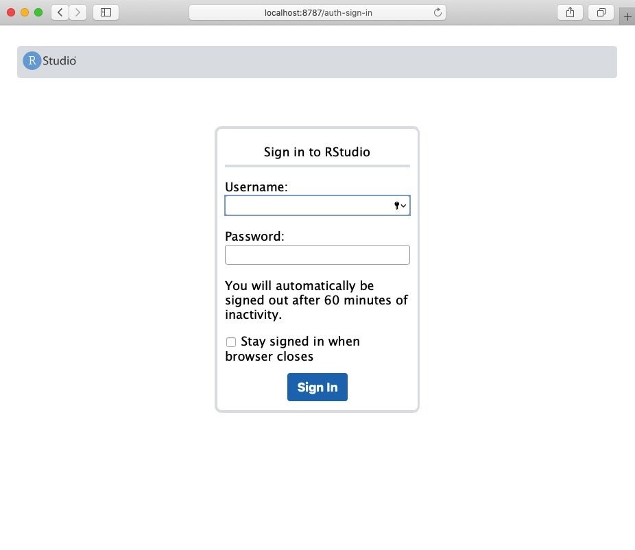
Now when you open localhost:8787 in a browser, you should see RStudio.

Sharon Machlis, IDG

The default user name and password are both rstudio, which of course would be terrible if you were running this in the cloud. But I think it’s fine on my local machine, since I don’t normally have any password on my regular RStudio desktop.

If you check the R version in your containerized R/RStudio, you’ll see it’s version 4.0. RStudio should be version 1.3.947, the latest preview release at the time this article first published. Those are both different versions from those installed on my local machine.

Three new R 4.0 features

So now let’s look at a few new features of R 4.0. 

New stringsAsFactors default

In the code below, I’m creating a simple data frame with info about four cities and then checking the structure.

City <- c("New York", "San Francisco", "Boston", "Seattle")
State <- c("NY", "CA", "MA", "Seattle")
PopDensity <- c(26403, 18838, 13841, 7962)
densities <- data.frame(City, State, PopDensity)
str(densities)
'data.frame':	4 obs. of  3 variables:
 $ City      : chr  "New York" "San Francisco" "Boston" "Seattle"
 $ State     : chr  "NY" "CA" "MA" "Seattle"
 $ PopDensity: num  26403 18838 13841 7962

Notice anything unexpected? City and State are character strings, even though I didn’t specify stringsAsFactors = FALSE. Yes, at long last, the R data.frame default is stringsAsFactors = FALSE. If I run the same code in an older version of R, City and State will be factors.

New color palettes and functions

Next, let’s look at a new built-in function in R 4.0: palette.pals(). This shows some built-in color palettes.

palette.pals()
 [1] "R3"              "R4"              "ggplot2"         "Okabe-Ito"      
 [5] "Accent"          "Dark 2"          "Paired"          "Pastel 1"       
 [9] "Pastel 2"        "Set 1"           "Set 2"           "Set 3"          
[13] "Tableau 10"      "Classic Tableau" "Polychrome 36"   "Alphabet"

Another new function, palette.colors(), gives info about a built-in palette.

palette.colors(palette = "Tableau 10")
     blue    orange       red lightteal     green    yellow    purple 
"#4E79A7" "#F28E2B" "#E15759" "#76B7B2" "#59A14F" "#EDC948" "#B07AA1" 
     pink     brown lightgray 
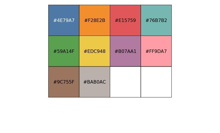
"#FF9DA7" "#9C755F" "#BAB0AC" 

If you then run the scales package’s show_col() function on the results, you get a nice color display of the palette.

scales::show_col(palette.colors(palette = "Tableau 10"))

Sharon Machlis, IDG

I made a small function combining the two that could be useful for looking at some of the built-in palettes in a single line of code:

display_built_in_palette <- function(my_palette) {
  scales::show_col(palette.colors(palette = my_palette))
}
display_built_in_palette("Okabe-Ito")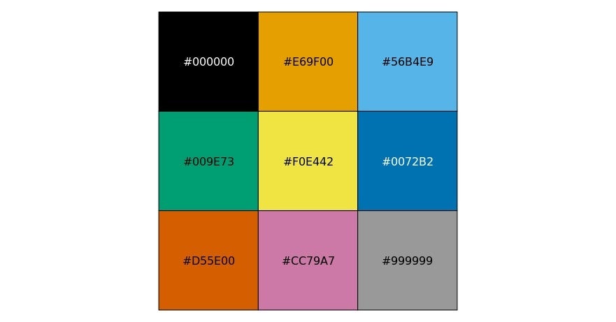

Sharon Machlis, IDG

None of this code works in earlier versions of R, since only scales::show_col() is available before R 4.0.

Escaping characters within strings

Finally, let’s look at a new function that makes it easier to include characters that usually need to be escaped in strings. 

The syntax is r"(my string here)". Here is one example:

string1 <-  r"("I no longer need to escape these " double quotes inside a quote," they said.)"

That string includes an un-escaped quotation mark inside a pair of double quotes. If I display that string, I get this:

> cat(string1)
"I no longer need to escape these " double quotes inside a quote," they said.

I can also print a literal \n inside the new function.

string2 <- r"(Here is a backslash n \n)"
cat(string2)
Here is a backslash n \n

Without the special r"()" function, that \n is read as a line break and doesn’t display.

string3 <- "Here is a backslash n \n"
cat(string3)
Here is a backslash n 

Before this in base R, you needed to escape that backslash with a second backslash. 

string4 <- "Usual escaped \\n"
cat(string4)
Usual escaped \n

That’s not a big deal in this example, but it can get complicated when you’re working on something like complex regular expressions.

There’s lots more new in R 4.0. You can check out all the details at the R project website. 

For more on using Docker with R, check out rOpenSci Labs’ short but excellent R Docker Tutorial.

And for more R tips, head to the InfoWorld Do More With R page!