R has a number of quick, elegant ways to join data frames by a common column. I’d like to show you three of them:
- base R’s
merge()function dplyr’s join family of functionsdata.table’s bracket syntax
Get and import the data
For this example I’ll use one of my favorite demo data sets—flight delay times from the U.S. Bureau of Transportation Statistics. If you want to follow along, head to http://bit.ly/USFlightDelays and download data for the time frame of your choice with the columns Flight Date, Reporting_Airline, Origin, Destination, and DepartureDelayMinutes. Also get the lookup table for Reporting_Airline.
Or, you can download these two data sets—plus my R code in a single file and a PowerPoint explaining different types of data merges—here:
To read in the file with base R, I’d first unzip the flight delay file and then import both flight delay data and the code lookup file with read.csv(). If you’re running the code, the delay file you downloaded will likely have a different name than in the code below. Also, note the lookup file’s unusual .csv_ extension.
unzip("673598238_T_ONTIME_REPORTING.zip")
mydf <- read.csv("673598238_T_ONTIME_REPORTING.csv",
       sep = ",", quote="\"")
mylookup <- read.csv("L_UNIQUE_CARRIERS.csv_",
            quote="\"", sep = "," )
Next, I’ll take a peek at both files with head():
head(mydf)
     FL_DATE OP_UNIQUE_CARRIER ORIGIN DEST DEP_DELAY_NEW  X
1 2019-08-01                DL    ATL  DFW            31 NA
2 2019-08-01                DL    DFW  ATL             0 NA
3 2019-08-01                DL    IAH  ATL            40 NA
4 2019-08-01                DL    PDX  SLC             0 NA
5 2019-08-01                DL    SLC  PDX             0 NA
6 2019-08-01                DL    DTW  ATL            10 NA

head(mylookup)
  Code                                          Description
1  02Q                                        Titan Airways
2  04Q                                   Tradewind Aviation
3  05Q                                  Comlux Aviation, AG
4  06Q                        Master Top Linhas Aereas Ltd.
5  07Q                                  Flair Airlines Ltd.
6  09Q Swift Air, LLC d/b/a Eastern Air Lines d/b/a Eastern
Merges with base R
The mydf delay data frame only has airline information by code. I’d like to add a column with the airline names from mylookup. One base R way to do this is with the merge() function, using the basic syntax merge(df1, df2). The order of data frame 1 and data frame 2 doesn't matter, but whichever one is first is considered x and the second one is y.
If the columns you want to join by don’t have the same name, you need to tell merge which columns you want to join by: by.x for the x data frame column name, and by.y for the y one, such as merge(df1, df2, by.x = "df1ColName", by.y = "df2ColName").
You can also tell merge whether you want all rows, including ones without a match, or just rows that match, with the arguments all.x and all.y. In this case, I’d like all the rows from the delay data; if there’s no airline code in the lookup table, I still want the information. But I don’t need rows from the lookup table that aren’t in the delay data (there are some codes for old airlines that don’t fly anymore in there). So, all.x equals TRUE but all.y equals FALSE. Here's the code:
joined_df <- merge(mydf, mylookup, by.x = "OP_UNIQUE_CARRIER",
             by.y = "Code", all.x = TRUE, all.y = FALSE)
The new joined data frame includes a column called Description with the name of the airline based on the carrier code:
head(joined_df)
  OP_UNIQUE_CARRIER    FL_DATE ORIGIN DEST DEP_DELAY_NEW  X       Description
1                9E 2019-08-12    JFK  SYR             0 NA Endeavor Air Inc.
2                9E 2019-08-12    TYS  DTW             0 NA Endeavor Air Inc.
3                9E 2019-08-12    ORF  LGA             0 NA Endeavor Air Inc.
4                9E 2019-08-13    IAH  MSP             6 NA Endeavor Air Inc.
5                9E 2019-08-12    DTW  JFK            58 NA Endeavor Air Inc.
6                9E 2019-08-12    SYR  JFK             0 NA Endeavor Air Inc.
Joins with dplyr
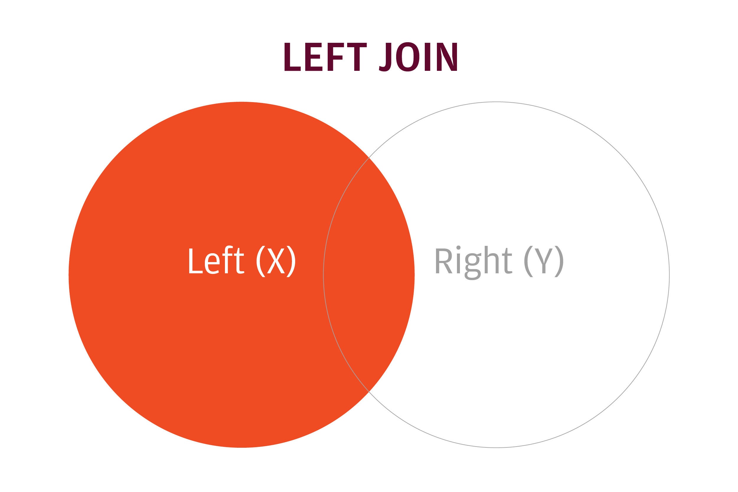
The dplyr package uses SQL database syntax for its join functions. A left join means: Include everything on the left (what was the x data frame in merge()) and all rows that match from the right (y) data frame. If the join columns have the same name, all you need is left_join(x, y). If they don’t have the same name, you need a by argument, such as left_join(x, y, by = c("df1ColName" = "df2ColName")).
Note the syntax for by: It’s a named vector, with both the left and right column names in quotation marks.
Update: Starting with dplyr version 1.1.0 (on CRAN as of January 29, 2023), dplyr joins have an additional by syntax using join_by():
left_join(x, y, by = join_by(df1ColName == df2ColName))
The new join_by() helper function uses unquoted column names and the == boolean operator, which package authors say makes more sense in an R context than c("col1" = "col2"), since = is meant for assigning a value to a variable, not testing for equality.
A left join keeps all rows in the left data frame and only matching rows from the right data frame.
The code to import and merge both data sets using left_join() is below. It starts by loading the dplyr and readr packages, and then reads in the two files with read_csv(). When using read_csv(), I don’t need to unzip the file first.
library(dplyr)
library(readr)
mytibble <- read_csv("673598238_T_ONTIME_REPORTING.zip")
mylookup_tibble <- read_csv("L_UNIQUE_CARRIERS.csv_")
joined_tibble <- left_join(mytibble, mylookup_tibble,
               by = join_by(OP_UNIQUE_CARRIER == Code))
Note that dplyr's older by syntax without join_by() still works
joined_tibble <- left_join(mytibble, mylookup_tibble,
              by = c("OP_UNIQUE_CARRIER" = "Code"))
read_csv() creates tibbles, which are a type of data frame with some extra features. left_join() merges the two. Take a look at the syntax: In this case, order matters. left_join() means include all rows on the left, or first, data set, but only rows that match from the second one. And, because I need to join by two differently named columns, I included a by argument.
The new join syntax in the development-only version of dplyr would be:
joined_tibble2 <- left_join(mytibble, mylookup_tibble,
              by = join_by(OP_UNIQUE_CARRIER == Code))
Since most people likely have the CRAN version, however, I will use dplyr's original named-vector syntax in the rest of this article, until join_by() becomes part of the CRAN version.
We can look at the structure of the result with dplyr’s glimpse() function, which is another way to see the top few items of a data frame:
glimpse(joined_tibble)
Observations: 658,461
Variables: 7
$ FL_DATE           <date> 2019-08-01, 2019-08-01, 2019-08-01, 2019-08-01, 2019-08-01…
$ OP_UNIQUE_CARRIER <chr> "DL", "DL", "DL", "DL", "DL", "DL", "DL", "DL", "DL", "DL",…
$ ORIGIN            <chr> "ATL", "DFW", "IAH", "PDX", "SLC", "DTW", "ATL", "MSP", "JF…
$ DEST              <chr> "DFW", "ATL", "ATL", "SLC", "PDX", "ATL", "DTW", "JFK", "MS…
$ DEP_DELAY_NEW     <dbl> 31, 0, 40, 0, 0, 10, 0, 22, 0, 0, 0, 17, 5, 2, 0, 0, 8, 0, …
$ X6                <lgl> NA, NA, NA, NA, NA, NA, NA, NA, NA, NA, NA, NA, NA, NA, NA,…
$ Description       <chr> "Delta Air Lines Inc.", "Delta Air Lines Inc.", "Delta Air …
This joined data set now has a new column with the name of the airline. If you run a version of this code yourself, you’ll probably notice that dplyr is way faster than base R.
Next, let’s look at a super-fast way to do joins.
Joins with data.table
The data.table package is best known for its speed, so it can be a good choice for dealing with large data sets.
In the code below, I load data.table and then use its fread() function to import the zip file. To read the zipped file, I use fread’s ability to call shell commands directly. That’s what the unzip -cq part of the argument is doing in the following fread()—you won't need that unless your file is zipped.
library(data.table)

mydt <- fread('unzip -cq 673598238_T_ONTIME_REPORTING.zip')
mylookup_dt <- fread("L_UNIQUE_CARRIERS.csv_")
fread() creates a data.table object—a data frame with extra functionality, especially within brackets after the object name. There are several ways to do joins with data.table.
One is to use the exact same merge() syntax as base R. You write it the same way, but it executes a lot faster:
joined_dt1 <- merge(mydt, mylookup_dt,
              by.x = "OP_UNIQUE_CARRIER", by.y = "Code",
              all.x = TRUE, all.y = FALSE)
If you want to use specific data.table syntax, you can first use the setkey() function to specify which columns you want to join on. Then, the syntax is simply mylookup_dt[mydt], as you can see in the code below:
setkey(mydt, "OP_UNIQUE_CARRIER")
setkey(mylookup_dt, "Code")
joined_dt2 <- mylookup_dt[mydt]
The creator of data.table, Matt Dowle, explained the format as “X[Y] looks up X rows using Y as an index.” But note that if you think of mylookup_dt as a lookup table, the lookup table is outside the brackets while the primary data is within the brackets.
There’s another data.table syntax that doesn’t require setkey(), and that’s adding an on argument within brackets. The syntax for the on vector is on = c(lookupColName = "dataColName"), with the lookup column name unquoted and the data column name in quotation marks:
dt3 <- mylookup_dt[mydt, on = c(Code = "OP_UNIQUE_CARRIER")]
Joins with dtplyr: dplyr syntax and data.table speed
I want to mention one other option: using dplyr syntax but with data.table on the back-end. You can do that with the dtplyr package, which is ideal for people who like dplyr syntax, or who are used to SQL database syntax, but want the speedy data.table performance.
To use dtplyr, you need to turn data frames or tibbles into special lazy data table objects. You do that with dtplyr’s lazy_dt() function.
In the code below, I use a %>% pipe to send the result of read_csv to the lazy_dt() function and then join the two objects the usual dplyr left_join() way:
my_lazy_dt <- readr::read_csv("673598238_T_ONTIME_REPORTING.zip") %>%
           dtplyr::lazy_dt()
my_lazy_lookup <- readr::read_csv("L_UNIQUE_CARRIERS.csv_") %>%
               dtplyr::lazy_dt()

joined_lazy_dt <- left_join(my_lazy_dt, my_lazy_lookup,
                  by = c("OP_UNIQUE_CARRIER" = "Code"))
As of this writing, dtplyr is not yet using the new by = joinby() syntax.
That joined_lazy_dt variable is a special dtplyr step object. If you print it, you can see the data.table code that created the object—look at the Call: line in the print() results below. That can be handy! You also see the first few rows of data, and a message that you need to turn that object into a data frame, tibble, or data.table if you want to use the data in there:
print(joined_lazy_dt)
Source: local data table [658,461 x 7]
Call:   setnames(setcolorder(`_DT5`[`_DT4`, on = .(Code = OP_UNIQUE_CARRIER),
    allow.cartesian = TRUE], c(3L, 1L, 4L, 5L, 6L, 7L, 2L)),
    "Code", "OP_UNIQUE_CARRIER")

  FL_DATE    OP_UNIQUE_CARRIER ORIGIN DEST  DEP_DELAY_NEW ...6  Description
  <date>     <chr>             <chr>  <chr>         <dbl> <lgl> <chr>
1 2019-08-01 DL                ATL    DFW              31 NA    Delta Air Lines Inc.
2 2019-08-01 DL                DFW    ATL               0 NA    Delta Air Lines Inc.
3 2019-08-01 DL                IAH    ATL              40 NA    Delta Air Lines Inc.
4 2019-08-01 DL                PDX    SLC               0 NA    Delta Air Lines Inc.
5 2019-08-01 DL                SLC    PDX               0 NA    Delta Air Lines Inc.
6 2019-08-01 DL                DTW    ATL              10 NA    Delta Air Lines Inc.
# … with 658,455 more rows
# ℹ Use `print(n = ...)` to see more rows

# Use as.data.table()/as.data.frame()/as_tibble() to access results
My complete code using a base R pipe:
joined_tibble <- left_join(my_lazy_dt, my_lazy_lookup,
                       by = c("OP_UNIQUE_CARRIER" = "Code")) |>
                 as_tibble()
After running some rather crude benchmarking several years ago, data.table code was fastest; dtplyr was almost as fast; dplyr took about twice as long; and base R was 15 or 20 times slower. Major caution here: that performance depends on the structure and size of your data and can vary wildly depending on your task. But it’s safe to say that base R isn’t a great choice for large data sets.
How to merge when you only want rows with matches
For the rest of these examples, I’m going to use two new data sets: Home values by U.S. zip code from Zillow and some population and other data by zip code from Simplemaps. If you’d like to follow along, download Median Home Values per Square Foot by Zip code from the Zillow research data page and the free basic database from Simplemaps' US Zip Codes Database page. (Because of licensing issues surrounding private data, these data sets are not included in the code and data download.)
In the code below, I’ve renamed files. If your data has different names or locations, adjust the code accordingly.
Base R and data.table
For both base R and data.table, if you want only rows that match, tell the merge() function all = FALSE. The code below reads in files and then runs merge() with all = FALSE:
# Import data
home_values_dt <- fread("Zip_MedianValuePerSqft_AllHomes.csv",
               colClasses = c(RegionName = "character"))
pop_density_dt <- fread("simplemaps_uszips_basicv1.6/uszips.csv",
               colClasses = c(zip = "character"))

# Merge data
matches1 <- merge(home_values_dt, pop_density_dt,
                  by.x = "RegionName",
                  by.y = "zip", all = FALSE)
Note that I set column classes as "character" when using fread() so that five-digit zip codes starting with 0 didn’t end up as four-digit numbers.
dplyr
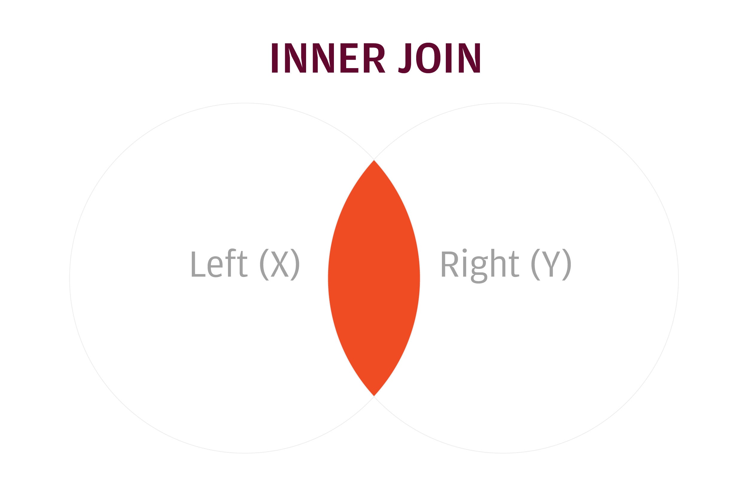
With dplyr, selecting only rows that match is an inner join:
The inner join keeps just rows that match in both data sets.
Here's the code:
# Import data
home_values <- read_csv("Zip_MedianValuePerSqft_AllHomes.csv")
pop_density <- read_csv("simplemaps_uszips_basicv1.6/uszips.csv")

# Merge data with inner join
matches2 <- inner_join(home_values, pop_density,
                       by = join_by(RegionName == zip))
# OR with older syntax:
matches2 <- inner_join(home_values, pop_density,
c("RegionName" = "zip"))
With readr’s read_csv(), the zip code columns automatically come in as character strings.
data.table bracket syntax
If you want to use data.table’s bracket syntax, add the argument nomatch=0 to exclude rows that don’t have a match:
matchesdt <- home_values_dt[pop_density_dt, nomatch = 0]
How to merge when you want all rows
Next, I'll show you the three ways to merge with all rows.
Base R and data.table
With base R or data.table, use merge() with all = TRUE:
all_rows1 <- merge(home_values_dt, pop_density_dt,
                   by.x = "RegionName", by.y = "zip", all = TRUE)
dplyr
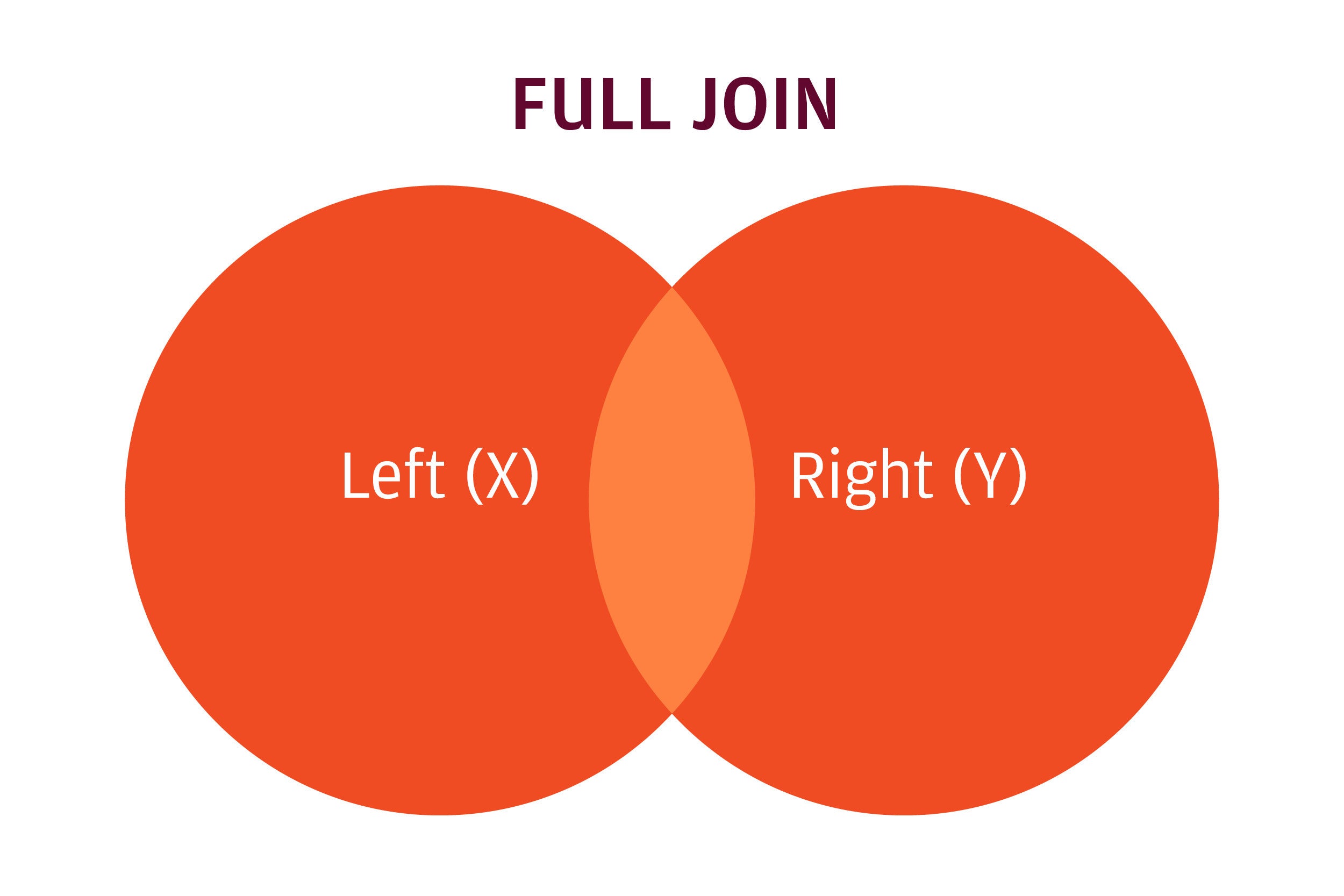
With dplyr, this is a full join:
The full join keeps all rows in both data sets.
all_rows2 <- full_join(home_values, pop_density,
                       by = join_by(RegionName == zip))
# OR
all_rows2 <- full_join(home_values, pop_density,
                       by = c("RegionName" = "zip"))
How to view rows in a data set without a match
It can be useful to check for rows in a data set that didn’t match, since that can help you understand the limitations of your data and whether something you expected is missing.
dplyr
In dplyr, finding rows that didn’t match is an anti join:
Anti join keeps rows from the left data frame without a match.
Here, as with left joins, order matters. To see all the rows in home_values without a match in pop_density, enter:
home_values_no_match <- anti_join(home_values, pop_density,
                         by = join_by(RegionName == zip))
# OR
home_values_no_match <- anti_join(home_values, pop_density,
                         by = c("RegionName" = "zip"))
And, to see all rows in pop_density that don’t have a match in home_values, it would be:
pop_density_no_match <- anti_join(pop_density, home_values,
                                  by = join_by(zip == RegionName))
data.table
While merge() syntax is fairly easy for most types of merges, in this case it gets a bit complex if you want rows without a match. I use dplyr’s anti_join() for this type of task, never merge().
If you want to use data.table bracket syntax, use this code to see all the rows in home_values_dt that don’t have a match in pop_density_dt:
home_values_no_match <- home_values_dt[!pop_density_dt]
Note that the code above assumes I’ve already run setkey() on both data sets. Pay attention to the order.
As we saw earlier, all rows in home_values, including those that have a match:
pop_density_dt[home_values_dt]
Only rows in home_values that don't have a match:
home_values_dt[!pop_density_dt]
Dowle’s full explanation to me about this syntax was: “X[Y] looks up X rows using Y as an index. X[!Y] returns all the rows in X that don’t match the Y index. Analogous to X[-c(3,6,10), ] returns all X rows except rows 3, 6, and 10.”
How to merge on multiple columns
Finally, one question I often see is, How do you combine data sets on two common columns?
merge()
To use merge() on multiple columns, the syntax is:
merge(dt1, dt2, by.x = c(”dt1_ColA", dt1_ColB"), by.y = c("dt2_cola", "dt2_colb"))
So, to merge home_values_dt and pop_density_dt on the zip code and city columns, the code is:
merge2_dt <- merge(home_values_dt, pop_density_dt,
                   by.x = c("RegionName", "City"),
                   by.y = c("zip", "city"),
                   all.x = TRUE, all.y = FALSE)
setting all.x and all.y as needed.
data.table
data.table has a couple of ways to set multiple keys in a data set. There’s setkey() to refer to column names unquoted, and setkeyv() if you want the names quoted in a vector (useful for when this task is within a function).
The formats are:
setkey(pop_density_dt, ZipCode, City)
# or
setkeyv(pop_density_dt, c("ZipCode", "City"))
And:
setkey(pop_density_dt, zip, city)
# or
setkeyv(pop_density_dt, c("zip", "city"))
Then, use your bracket syntax as usual, such as:
pop_density_dt[home_values_dt]
dplyr join_by() syntax is
join_by(id1 == id2, colA == colB)
Want more R tips? Head to the Do More With R page!