How to do spatial analysis in R with sf

Where do you vote? Who are you legislators? What is your ZIP code? These questions have something geospatially in common: The answer involves determining which polygon a point falls within.

Such calculations are often done with specialized GIS software. But they’re also easy to do in R. You need three things:

1. A way to geocode addresses to find latitude and longitude; 
2. Shapefiles that outline ZIP code polygon boundaries; and 
3. The sf package.

For geocoding, I usually use the geocod.io API. It’s free for 2,500 lookups a day and has a nice R package, but you need a (free) API key to use it. To get around that bit of complexity for this article, I’ll use the free, open-source Open Street Map Nominatim API. It doesn’t require a key. The tmaptools package has a function, geocode_OSM(), to use that API.

Importing and prepping geospatial data

I’ll be using the sf, tmaptools, tmap, and dplyr packages. If you want to follow along, load each with pacman::p_load() or install any not yet on your system with install.packages(), then load each with library().

For this example, I’ll create a vector with two addresses, our IDG office in Framingham, Massachusetts, and the RStudio office in Boston.

addresses <- c("492 Old Connecticut Path, Framingham, MA", 
               "250 Northern Ave., Boston, MA")

Geocoding is straightforward with geocode_OSM. You can see the results by printing out the first three columns including latitude and longitude:

geocoded_addresses <- geocode_OSM(addresses)
print(geocoded_addresses[,1:3])
                                     query      lat       lon
# 1 492 Old Connecticut Path, Framingham, MA 42.31348 -71.39105
# 2            250 Northern Ave., Boston, MA 42.34806 -71.03673

There are several ways to get ZIP code shapefiles. The easiest is probably the U.S. Census Bureau’s ZIP Code Tabulation Areas, which are similar to if not exactly the same as U.S. Postal Service boundaries.

You can download a ZCTA file directly from the U.S. Census Bureau, but it’s a file for the entire country. Only do that if you don’t mind a large data file. 

One place to download a ZCTA file for a single state is Census Reporter. Search for any data by state, such as population, and then add ZIP code to the geography and choose download data as a shapefile.

I could unzip my downloaded file manually, but it’s easier in R. Here I use base R’s unzip() function on a downloaded file, and unzip it to a project subdirectory named ma_zip_shapefile. That junkpaths = TRUE argument says I don’t want unzip adding another subdirectory based on the name of the zip file.

unzip("data/acs2017_5yr_B01003_86000US02648.zip", 
      exdir = "ma_zip_shapefile", junkpaths = TRUE, 
      overwrite = TRUE)

Geospatial import and analysis with sf

Now finally some geospatial work. I’ll import the shapefile into R using sf’s st_read() function.

zipcode_geo <- st_read("ma_zip_shapefile/acs2017_5yr_B01003_86000US02648.shp")
# Reading layer `acs2017_5yr_B01003_86000US02648' from data source `/Users/smachlis/Documents/MoreWithR/ma_zip_shapefile/acs2017_5yr_B01003_86000US02648.shp' using driver `ESRI Shapefile'
# Simple feature collection with 548 features and 4 fields
# geometry type:  MULTIPOLYGON
# dimension:      XY
# bbox:           xmin: -73.50821 ymin: 41.18705 xmax: -69.85886 ymax: 42.95774
# epsg (SRID):    4326
# proj4string:    +proj=longlat +datum=WGS84 +no_defs

I’ve included the console response when running st_read() because there’s some information displayed there: the epsg. That says what coordinate reference system was used to create the file. Here it was 4326. Without getting too deep into the weeds, an epsg basically indicates what system was used to translate areas on a three-dimensional globe—the Earth—to two-dimensional coordinates (latitude and longitude). This is important because there are a lot of different coordinate reference systems. I want my ZIP code polygons and address points to use the same one, so they line up properly.

Note: This file happens to include a polygon for the entire state of Massachusetts, which I don’t need. So I’ll filter out that Massachusetts row with

zipcode_geo <- dplyr::filter(zipcode_geo, 
                             name != "Massachusetts")

Mapping the shapefile with tmap

Mapping the polygon data isn’t necessary, but it’s a nice check of my shapefile to see if the geometry is what I expect. You can do a quick plot of an sf object with tmap’s qtm() (short for quick theme map) function.

qtm(zipcode_geo) +
  tm_legend(show = FALSE)

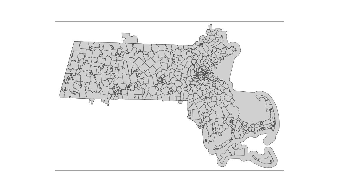Screens shot by Sharon Machlis, IDG

And it looks like I do indeed have Massachusetts geometry with polygons that could be ZIP codes.

Next I want to use the geocoded address data. This is currently a plain data frame, but it needs to be converted into an sf geospatial object with the right coordinate system.

We can do that with sf’s st_as_sf() function. (Note: sf package functions that operate on spatial data start with st_, which stands for “spatial” and “temporal.”)

st_as_sf() takes several arguments. In the code below, the first argument is the object to transform—my geocoded addresses. The second argument vector tells the function which columns have the x (longitude) and y (latitude) values. The third sets the coordinate reference system to 4326, so it’s the same as my ZIP code polygons.

point_geo <- st_as_sf(geocoded_addresses, 
                      coords = c(x = "lon", y = "lat"), 
                      crs = 4326)

Geospatial joins with sf

Now that I’ve set up my two data sets, calculating the ZIP code for each address is easy with sf’s st_join() function. The syntax:

st_join(point_sf_object, polygon_sf_object, join = join_type)

In this example, I want to run st_join() on the geocoded points first and the ZIP code polygons second. It’s a so-called left join format: All points in the first data (geocoded addresses) are included, but only points in the second (ZIP code) data that match. Finally, my join type is st_within, since I want the match to be points within. 

my_results <- st_join(point_geo, zipcode_geo, 
                      join = st_within)

That’s it! Now if I look at my results by printing out several of the most important columns, you”ll see each address has a ZIP code (in the “name” column). 

print(my_results[,c("query", "name", "geometry")])
# Simple feature collection with 2 features and 2 fields
# geometry type:  POINT
# dimension:      XY
# bbox:           xmin: -71.39105 ymin: 42.31348 xmax: -71.03673 ymax: 42.34806
# epsg (SRID):    4326
# proj4string:    +proj=longlat +datum=WGS84 +no_defs
#                                      query  name                   geometry
# 1 492 Old Connecticut Path, Framingham, MA 01701 POINT (-71.39105 42.31348)
# 2            250 Northern Ave., Boston, MA 02210 POINT (-71.03673 42.34806)

Mapping points and polygons with tmap

If you’d like to map the points and polygons, here’s one way to do it with tmap:

tm_shape(zipcode_geo) +
tm_fill() +
tm_shape(my_results) +
tm_bubbles(col = "red", size = 0.25)

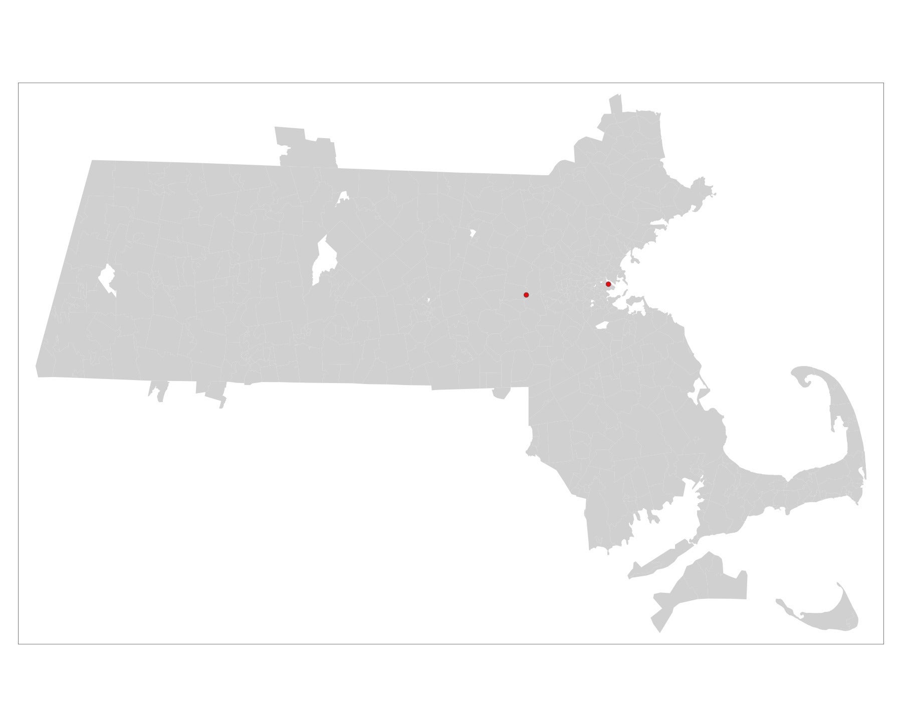Screen shot by Sharon Machlis, IDG

Want more R tips? Head to the “Do More with R” page!